- Research
- Open access
- Published:
Cubic time algorithms of amalgamating gene trees and building evolutionary scenarios
Biology Direct volume 7, Article number: 48 (2012)
Abstract
Background
A long recognized problem is the inference of the supertree S that amalgamates a given set {G j } of trees G j , with leaves in each G j being assigned homologous elements.
We ground on an approach to find the tree S by minimizing the total cost of mappings α j of individual gene trees G j into S. Traditionally, this cost is defined basically as a sum of duplications and gaps in each α j . The classical problem is to minimize the total cost, where S runs over the set of all trees that contain an exhaustive non-redundant set of species from all input G j .
Results
We suggest a reformulation of the classical NP-hard problem of building a supertree in terms of the global minimization of the same cost functional but only over species trees S that consist of clades belonging to a fixed set P (e.g., an exhaustive set of clades in all G j ). We developed a deterministic solving algorithm with a low degree polynomial (typically cubic) time complexity with respect to the size of input data.
We define an extensive set of elementary evolutionary events and suggest an original definition of mapping β of tree G into tree S. We introduce the cost functional c(G, S, f ) and define the mapping β as the global minimum of this functional with respect to the variable f, in which sense it is a generalization of classical mapping α.
We suggest a reformulation of the classical NP-hard mapping (reconciliation) problem by introducing time slices into the species tree S and present a cubic time solving algorithm to compute the mapping β. We introduce two novel definitions of the evolutionary scenario based on mapping β or a random process of gene evolution along a species tree.
Conclusions
Developed algorithms are mathematically proved, which justifies the following statements. The supertree building algorithm finds exactly the global minimum of the total cost if only gene duplications and losses are allowed and the given sets of gene trees satisfies a certain condition. The mapping algorithm finds exactly the minimal mapping β, the minimal total cost and the evolutionary scenario as a minimum over all possible distributions of elementary evolutionary events along the edges of tree S.
The algorithms and their effective software implementations provide useful tools in many biological studies. They facilitate processing of voluminous tree data in acceptable time still largely avoiding heuristics. Performance of the tools is tested with artificial and prokaryotic tree data.
Reviewers
This article was reviewed by Prof. Anthony Almudevar, Prof. Alexander Bolshoy (nominated by Prof. Peter Olofsson), and Prof. Marek Kimmel.
Background
Problems in supertree inference
Denote S a tree of species or other taxonomic units, proteins, etc. The long recognized problem is to infer a tree S that amalgamates a given set {G j } of trees G j , with leaves in each G j being assigned homologous sequences from an j-th family of homologous elements. Only leaf names, not sequences themselves, are considered. Henceforth, assume that leaves in S are labeled with species names x, leaves in each G j – with species-gene names x-y (gene “y” exists in species “x”); paralogs are allowed. Refer to S as a species tree, and to each G j as a gene tree.
We elaborate a traditional approach from [1, 2] to find the tree S such that it minimizes the total cost of mappings of individual gene trees G j into S.
Traditionally, some cost c(G S) of mapping of a gene tree G into a species tree S is defined. Choosing a particular definition of c(G S) (ref. e.g. to [2, 3] and see Results) is not essential in terms of solving the classical problem below. For a given set {G j } of gene trees the total cost is defined as
where k j are certain weights. The classical problem is to find such S that globally minimizes the functional c({G j },S), where S runs over the set of all species trees that contain an exhaustive non-redundant set of species from all input G j . Such S is called a supertree for the given set {G j }. Denote V0 a set of all species names occurring in leaves of the input trees G j . Thus, the classical problem is to find the global minimum of cost functional (1) over all species trees S that possess the set V0 of leaf names.
The supertree building problem is NP-hard, i.e., any algorithm to solve it must possess an exponential complexity (if NP ≠ P). Numerous heuristics exist (e.g. in [4–6]), which however do not provide evaluations of the runtime of corresponding algorithms. Unless NP = P, none of them can possess a polynomial complexity and be proved to find the true global minimum.
We propose a reformulation of the classical problem and develop an effective deterministic algorithm that meets many biological prerequisites (Description of the first algorithm and Results). Namely, the supertree S is sought for as a global minimum of (1) but S runs over a set of such species trees that mostly contain clades present in input trees G j , [3, 7, 8]. A set of species names assigned to leaves of a subtree in G j with the root v is called a clade (of vertex v in G j ) and denoted by cl(v). The set P includes all clades from trees G j and additionally the set of species names V0. Such P is referred to as a standard set. Its cardinality has the order of nm, where n is the number of gene trees, and m is the total number of species. For the standard set P, the algorithm’s running time is cubic and determined by formula (2) below.
Further, suppose that cl(v1), cl(v2) are the clades of two noncomparable vertices v1, v2 in a tree G j , and the intersection I(v1v2) of these clades is not empty. Optionally, the sets cl(v i ) – I(v1v2), (i=1, 2) are also included in P; and for each vertex v that is ancestral to v i (i=1 or i=2) but not to another vertex from the pair v1, v2, the set cl(v) – cl(v i ) is included in P. In so doing, horizontal gene transfers are accounted for in a species tree, ref. to [9].
If P includes any other nonempty subsets of V0 and its cardinality is arbitrary, the algorithm remains cubic in time but with respect to cardinality |P| of set P, ref. to formula (3) below.
Therefore, the non-standard problem formulated in this study consists of finding the global minimum of functional (1) among species trees S that have the set of leaves V0 and a set of clades belonging to a fixed set P. Thus, P is a parameter of the problem and of the solving algorithm. The algorithm operates equally with any P. The solution is also referred to as a supertree or a “limited supertree” with respect to P.
A mapping of G j into S, as well as defyning any scenario, requires a pre-defined fixed set of elementary evolutionary events. The standard set (of events) contains only gene duplications and losses. The extended set (of events) additionally contains horizontal gene transfers, gains, etc. The list of elementary evolutionary events and their definitions are given in Description of the first algorithm. Henceforth, edges in a species tree are referred to as tubes to contrast the difference with the edges in gene trees.
With the standard event set, the algorithm possesses the running time of
For simplicity, here we assume that the average number of leaves in given trees G j is multiple of m.
If set P has an arbitrary cardinality, the mentioned time has the order of
Let a set {G j } of gene trees and its associated P be fixed. A set V∈P is defined as basic if it is either a singleton set or can be split into two basic sets. Let us introduce the condition
“V0 is a basic set” (*)
The condition imposes a certain dependency between sets {G j }, P and V0.
With the standard event set and condition (*), the algorithm was mathematically proved [7], which means that it outputs the true global constrained minimum of the corresponding functional.
It is difficult, however, to mathematically prove the algorithm for the case of the extended event set and/or a relaxation of condition (*). We believe that including horizontal gene transfers still produces valid results [7], and/or condition (*) can be relaxed.
The authors are unaware from published literature of analogous approaches to find a mathematically proved supertree in cubic time.
In Testing of the algorithms we present testing of the supertree building algorithm with artificial and biological data.
A relevant biological discussion of our approach is provided in [8]. The mapping cost in [3] is similar to the cost from [2] in the case of standard event set.
Problems in inferring evolutionary scenario
Patterns of gene evolution possess a number of various types of events that co-occur with the species evolution. Identification of these types and assembling elementary events into an evolutionary scenario is crucial for understanding the evolutionary histories of genes, genomes, species, and higher taxonomic lineages, ref. e.g. to [10–12]. Important is to create a model that incorporates all known event types, as well as a model of co-evolution of regulatory systems, genes and species, e.g. [13]. Studies (e.g. in [14]) show the importance of considering suboptimal (in terms of the total cost) solutions in searches, as those might represent optimal scenarios when the costs of elementary events are slightly varied. This problem is partially tackled in Second scenario design: a random process on the graph.
In pioneer papers [2], the cost c0(G S) is defined through the mapping α(G, S) of a given tree G into S basically as a sum of duplications (pairs <x, z>, where α(x)=α(z)) and gaps (vertices y, where there is no x for which y=α(x)). For the given G and S, the mapping α can be computed as a global minimum of the functional c0(G S f) that depends on the variable f running over a suitable set of mappings f of G into S; such α can be obtained in linear time with respect to the size of input data, and c0(G,S) becomes equal to c0(G, S, α). Definitions of the cost and mapping are closely related to the definition of the evolutionary scenario, i.e., a pattern of elementary evolutionary events that a gene undergoes along the branches of tree S. An important part of this definition is the choice of allowed elementary evolutionary events and their costs. In [2] the list included only gene duplications and losses. We consider the extended set of elementary evolutionary events listed in the Methods, and the novel definition of cost c(G,S) (see Computing the total cost of binary gene trees against the species tree).
If horizontal gene transfers are allowed, any mapping algorithm suffers from an intrinsic prohibition of gene transfers across different levels of the species tree. If this prohibition holds, the problem of building the globally minimal (i.e., globally minimizing the cost functional) mapping of G into S is NP-hard.
In order to circumvent the NP-hard nature of the problem and develop a polynomial time algorithm to solve it, the concept of time slices in species tree S was introduced [3, 15, 16]. This concept is in some sense related to an earlier approach to date tree vertices [17]. The concept is biologically justified, although its correct definition is still to be developed.
More precisely, edges of S can be broken by inserting additional vertices, thus formally producing another tree S0, Figure 1; in the special case S=S0. It imposes time slices in S such that any horizontal transfers are allowed but only within one slice. The algorithm of building time slices [3, 15] constructs the tree S0 such that the k-th slice contains all edges distant by the amount of k edges from the root. Naturally, any two consecutive edges in S0 belong to different slices.

A transition from tree S to tree S 0 . Leaves 1, 2, 3 contain in-group species, leaf d* contains an auxiliary outgroup species. Leaf d* is connected to the root by the outgroup tube (shown in bold). All tubes acquire additional vertices during transition to S0 (right, shown in bold) to delimit time slices (here four slices are separated by dashed lines). Each slice thus contains one segment of the outgroup tube in S (left), which forms the outgroup tubes in S0 (each shown in bold). Any such segment, as well as the outgroup leaf-species, are denoted as d*. The root tube d0 is attached to the root, by analogy with the edge e0 in a gene tree G.
Recall that edges in S0 and S are referred to as tubes to contrast the difference with the edges in gene trees; inserted vertices split a tube into a succession of new tubes.
The generalization of mapping α is proposed for the case of the extended set of elementary evolutionary events listed in Description of the first algorithm. This generalization denotes the mapping β. Its definition and details of computing are provided under First scenario design: the event tree. Equivalently, β can be defined as the global minimum of the cost c(f) over a set of mappings f of G into S0 (this definition is not provided).
We developed an algorithm that reconciles any gene tree G and tree S0, i.e., computes a rigorous (mathematically proved) minimal mapping β of G into S0 in time O(|G|×|S0|), which gives O(|S|3) for the time slices building algorithm from [3, 15]. Recall that | | is the cardinality of a corresponding set; in terms of trees it is the cardinality of the set of vertices. As above, for simplicity we assume that the average number of leaves in G is multiple of m. The “mathematically proved” means that β is the true global minimum of the cost c(f). The mathematical proof is given in [3, 13], and is reproduced with definitions from [3, 13] in the later paper [18].
Note that in [16] the biologically important case of the loss of a horizontally transferred gene in the donor (in that study, the case cannot be reduced to a composition of events) is not considered, and the study claims a polynomial runtime of the algorithm yet not specifying the polynomial degree.
Objectives
One block of objectives is: (i) to formulate the problems and hypotheses in building supertrees and evolutionary scenarios, (ii) to describe the algorithm of solving the non-standard problem of building a supertree (referred to as the first algorithm) and to introduce the Super3GL program that implements the algorithm [19] (See Description of the first algorithm and Results), (iii) to compare the program with known supertree inferring tools (Testing of the algorithms).
We describe comparisons with two recognized computer programs in Implementation of the second algorithm, testing against other well-known software tools produced similar results. A rigorous comparison using artificial data implies having a sound algorithm to simulate gene trees on a known species tree topology. This problem needs further research and justification, however a particular algorithm was proposed in [8].
The next block objectives is: (iv) to present the concept of the evolutionary scenario based on either mapping β or a random process of gene evolution (see First scenario design: the event tree - Stochastic characteristics of the second scenario design), (v) to describe solutions to concomitant problems, viz. computing the originally introduced cost c(G S) (see Conclusion) and the transition from a polytomous tree to the corresponding binary tree (the “binarization” operation). For convenience, these algorithms in complex are referred to as the second algorithm. Implementation of the first algorithm and Implementation of the second algorithm detail the implementations of the first and second algorithms, accordingly [19, 20].
Methods
Description of the first algorithm
The algorithm is applicable to both an arbitrary set of evolutionary events and an arbitrary set P. In this general case the algorithm is heuristic and is tested in Testing of the algorithms (data partially shown). As noted in the Background, the exact condition necessary and sufficient for the algorithm to be mathematically proved is unknown to the authors.
Given is a set of rooted gene trees G j with allowed polytomies. To pre-process unrooted trees, a simple php script was developed to root trees. The script is available at the Web page [19] and its description is given in Additional file 1.
The first algorithm consists of two phases:
-
I.
building the set {S(V)| V}, where the variable V runs over all basic sets (ref. to the Background), and S(V) is the corresponding (to a given V) basic tree (this notion is explained below);
-
II.
assembling the set of basic trees S(V) into the sought-for supertree S*.
Phase I is rigorous (mathematically proved), at least when only gene duplications and losses are considered, and condition (*) is true. However, we operate with the full set of elementary evolutionary events (see Table 1 below), in which case the algorithm is heuristic.
If V0 is a basic set then S(V0) can already be considered an outcome of the algorithm (omitting Phase II). However, our experiments show that engaging Phase II improves the result quality.
-
I)
The first phase (Phase I) consists of five steps:
-
I.1)
Optional tree pruning. An inextensible subtree of G j with all leaves belonging to a species s is called the occurrence of species s (in G j ). For each species s that occurs less than p times (a parameter of the algorithm) in the given set {G j } of gene trees, every gene of this species is removed from all G j . After such trimming in each G j “pendant” edges are removed together with their origins. Next, all gene trees that become empty or contain only one species are also removed. Such a reduced set of gene trees is still denoted by {G j }. This step is trivial but might be useful.
-
I.2)
Composing the set P of species sets. The set P (refer to its definition in the Background) is built and ordered by ascending the cardinality of constituent sets.
-
I.3)
Constructing the set of “good” vertices. Let G j be binary. Given a set V ? P, a non-root vertex v of tree G j is called good (with respect to V) if
(4)where v' is the parent vertex of v. The root of the tree is considered good if the first condition in (4) is true. Now let G j be polytomous. We assume that G j contains an additional edge e0 located upwards from the root as shown in Figure 2. Given a set V ∈ P, a vertex v of tree G j is called good (with respect to V) if at least one of its children obeys condition (4) or the first condition in (4) if v is the super-root. For each set V ∈ P, the set R(V) of good vertices in all source gene trees G j is composed. If a binary tree G j is also considered polytomous, these two definitions give, generally defining, different sets of good vertices but of equal cardinality. It is enough, as only the cardinality of the set R(V) is considered further.
Figure 2 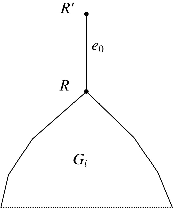
An additional “root” edge between the “super-root” R' and the initial root R in tree G j . This root is used to define the set R(V), since the vertex R' can be good. The root edge e0 is analogous to the root tube d0 in Figure 1.
-
I.4)
Finding basic sets and their partitions in the set P. For each fixed non-singleton basic set V (in P), all partitioning variants are considered, i.e., all variants defined by the equality V = V1+V2, where non-empty disjoint sets V1, V2 are themselves basic.
-
I.5)
Building basic trees S(V) and computing their costs. For each basic set V, the basic tree S(V) along with its cost c(V) is defined and computed by induction. The tree S(V) for a singleton set V consists of one root-leaf vertex assigned a species from V; the cost c(V) of this S(V) is zero. The induction step for a fixed V: for each partition variant V = V1+V2 the value c(V1,V2) = c(V1) + c(V2) + C d + C l is computed, and the minimum (over all partitions of V).
-
I.1)

is found, where C d is the total cost of duplications on edge V (we equally denote by V the set of leaf species, the root edge and the root vertex of the corresponding subtree), and C l is the total cost of losses on edges V1 and V2, see Figure 3. Both C d and C l are defined below.

Tree S ( V ) for a fixed partition V = V 1 + V 2 . Here V, V1, V2 designates both the corresponding vertex and the edge upwards from this vertex. Trees S(V1) and S(V2), as well as their costs c(V1) and c(V2), are already known from induction, and C d + C l corresponds to evolutionary events in edges of V, V1, V2. Those are not known from induction and should be computed separately, as defined below in the text.
A partition <V1,V2> that minimizes the functional c(V) over all partitions of V is called the minimal partition (of V). Once the minimal partition is found, the tree S(V) is obtained by joining trees S(V1) and S(V2) and rooting them at the joint vertex and edge, as shown in Figure 3.
Thus, to calculate the total costs C d and C l , a set r(V1,V2) of vertices v in all G j is constructed such that one child vertex of v belongs to R(V1), and the other – to R(V2) (if v is binary). A polytomous vertex v is included in r(V1,V2) if v possesses at least one child satisfying (4) for V1 and one satisfying (4) for V2. The total cost of duplications on edge V is calculated as C d = c d · (|R(V1)|+|R(V2)|–|R(V)|–|r(V1,V2)|), where | | denotes the cardinality of a set, and c d is the cost of one duplication (the algorithm parameter). The total cost of losses in edges V1 and V2 is calculated as C l = c l · (|R(V1)|+|R(V2)|–2|r(V1,V2)|), where c l is the cost of one loss (the algorithm parameter).
Additionally, the weight of the tree S(V) is calculated with the formula
where a is the number of leaves in S(V), m is the total number of species, and c is the algorithm parameter (default is c=10). Here the partition V' is closest to the minimal partition in terms of the cost; if no other partition exists, it is assumed that w(V) = 1. The weights are used at Phase II of the algorithm.
Phase I (steps I.1-I.5) ends with removing all basic trees containing less than 3 leaves. The obtained set of weighted basic trees is the outcome of Phase I of the first algorithm.
Operating time of Phase I for the standard P has the order of O((n·m)3), and for any P – the order is O(|P|3 + |P|2nm). A rigorous cubic complexity and mathematical proof (in the special common case) are the advantages of the Phase I algorithm comparing to known heuristic methods.
II) The second phase of the first algorithm (Phase II). This phase is heuristic. For any species tree S with the leaves-species set W and the basic tree S(V), define the cost c(S(V),S) as the cost of mapping α or β of the tree S'(V) into S (the cost of β is defined in see Computing the total cost of binary gene trees against the species tree below). Here, S'(V) is obtained from S(V) by pruning all leaves containing species outside W together with their edges.
The cost c(S) of any species tree S is defined as the sum of costs c(S(V),S) over all basic trees S(V), or, optionally, each cost is multiplied by w(V). Thus,
where summation is done over all basic trees S(V) or, equally, over all basic sets V with cardinality higher than or equal to 3. As above, let V0 be the set of all species contained in leaves of all G j .
The initial step of Phase II. The algorithm enumerates all triplet-leaved trees S with three leaves-species from V0 and selects one with the minimal cost c(S). This S constitutes the seed partial supertree in the below procedure.
The inductive step of Phase II. In the current partial supertree S with the set W of leaves-species (a subset of V0), each edge is attempted for insertion of a new vertex a connected to a species s from V0, and for placing a new root a above the current root, Figure 4. Among such possible extensions T of S, we choose the tree T with the minimal cost с(T); it supersedes the current partial supertree S. Extensions are attempted until all species from V0 are added to the current tree S, and the algorithm halts. The eventual S is the sought-for supertree S*. The end of Phase II.

Two possibilities of inserting a new vertex a connected by an edge with a new species s.
Additional file 1 contains a more detailed description of Phase II, including the assessment of vertex reliability in the final supertree and overall supertree reliability. It also presents a simplified version of Phase II.
The second algorithm: reconciliation of gene and species trees and building evolutionary scenarios
Given are a set {G j } of rooted polytomous gene trees (paralogs are allowed), a rooted binary species tree S and a tree S0 obtained from S by inserting one or several vertices into tubes to delimit time slices, Figure 1. Each G j and the tree S0 are attributed the root edge e0 and the root tube d0 as depicted in Figure 2. If the index j is irrelevant, G j is equivalent to G.
The set of species is fixed, with one “accessory” outgroup leaf d* added to the tree root. For the species tree, the notations of terminal tubes, leaves and species x (including the outgroup) are unified to define identical objects. For gene trees, the identical objects are terminal edges, leaves and leaf notations x-y. The correspondence between leaf notations x-y in G and x in S and S0 is fixed as the gene-species correspondence (gene “y” exists in species “x”).
The second algorithm refers to a complex of algorithms to solve four separate problems as described below in Computing the total cost of binary gene trees against the species tree - Stochastic characteristics of the second scenario design.
Ordering used in the algorithm
All gene trees G j are enumerated (index j can be omitted). Under a fixed j, triplets < e,d,i > are enumerated as follows. Edges e in G are visited in the order of descending distance from the root (from deeper to shallower levels), and from left to right within the same level. Tubes d in S0 are visited in the order of descending the level of the time slice (upwards to the root). Within a slice, for each e ≠ e0 tubes are visited from left to right starting from the outgroup d*, and for the root edge e0 the left-to-right visiting ends with the outgroup d*. Here d* is a segment of the outgroup tube in tree S that falls within the current time slice. Next, the 35 types of gene evolution events i are visited in the order specified in Table 1, with i running from 0 to 34.
All trees G considered (see Conclusion) are binary. Encountered polytomous trees are binarized. The binarization procedure is described in Additional file 2.
Computing the total cost of binary gene trees against the species tree
In Table 1, each row provides the event name and description (third and fourth columns, respectively), and the last column defines the cost of <e,d,i>.
Let j specify the tree G, e run over its edges, and d run over tubes in S0. Define
where с(e,d,i) is the cost specified in the last column of Table 1 if the current pair <e,d> satisfies the condition defining the particular event type. In computing сmin(e,d) the arguments <e,d> are enumerated according to the ordering specified in The second algorithm: reconciliation of gene and species trees and building evolutionary scenarios. Figure 5 exemplifies an induction step.

The inductive step in computing the cost c ( G , S ). On the left is an illustration of assembling the tree G from subtrees G1 and G2. Here е1 is the root edge in G1, е2 – the root edge in G2 (the root edges belong to their corresponding trees), and е – the root edge in G. Figure on the right illustrates an embedding of G into S. Costs c(G1,S) and c(G2,S) are computed with induction. Then c(G,S) = c(G1,S) + c(G2,S) + x, here х=с(loss)+c(transfer)+c(dupl), and summands are parameters of the algorithm (elementary event costs).
The minimum of (5) is attained at the “minimal” event (the “minimal” row in Table 1) i. Certain events imply the minimization over the variable tube d' or the pair of tubes <d',d">; the minimal value of the variable is referred to as the “minimal parameter”.
The value сmin(e0, d0) is denoted as c(G, S), recall that G = G j . The value is denoted as c({G j }, S) and referred to as the total cost of the input set {G j } of binary gene trees against the tree S. The total cost of the supertree S* is denoted as c({G j }, S *).
The value сmin(e, d) can be interpreted as a “conditional cost”, i.e. the cost of an optimal evolutionary scenario if it initiates from edge e in tube d and evolves into terminal leaves with cohered pairs of genes-species.
First scenario design: the event tree
Each tree G (or its binarization G') is associated with the first scenario (the event tree) T of the evolution of gene G along the species tree S0. The tree vertices correspond to certain pairs <e,d>, the root – to the pair <e0,d0>, the leaves – to pairs formed with a terminal edge and a terminal tube obeying the “species-gene” relation. The tree edges can be unary (ordinary) or binary, i.e., pairs of unary edges originated from a single vertex. The algorithm of constructing T over G is similar to the binarization procedure detailed in Additional file 2.
During the forward run (described in Computing the total cost of binary gene trees against the species tree) each pair <e,d> is assigned the minimal event i according to (5) and its minimal parameters. The backward run starts from the pair <e0,d0>. At each step either a binary edge is projected from vertex <e,d> into vertices denoted as <е1,d'1> and <е2,d'2> (case 1), or a unary edge is projected into vertex <e,d'> (case 2), where d'1, d'2, d' are the minimal parameters. The edge is tagged with the event name i. Case 1 implies a bifurcation resulted from the minimal event.
By definition, the cost of the first scenario T is the cost of the input tree G against S0, i.e. c(T) = c(G, S0). It can be detailed with the amounts of different event types inferred in tubes of the species tree, the total amount of events, the individual event costs, etc.
The mapping β is equivalent to T , and the cost of β is equal to the cost of T as substantiated below. It is easy to show that for each е in G there are vertices in T of the form < e, d > with different tubes d. Each such tube d1,…, d l is associated in T with the unique corresponding event i t that occurred on edge e inside tube d t (such i t tags the unique edge originated from vertex < e, d t > in T). By definition, β(e)={d1, …, d t ,…, d l }. The set β(e) can be interpreted as a path. Consider first d1 that is closest to the root in S0. If tubes d t and dt+1 are comparable then d t is closer to the root, otherwise dt+1 accepts a transfer from d t (Figure 6) or dt+1 is a child of the accepting tube. The set β(e) forms in S0 a connected path defined by the scenario T and consisting of repetitions of edge e and transfers without retention. This definition of β(e) requires a clarification: events i t are determined by β(e) and S0, except for the last event i l . Therefore, β(e) can be expressed as β(e)={d1, …, d l ; i l }. For mapping β let us define c(β) = c(T).

An example of β ( e ) value. Edge e may cross different time slices (not shown), undergoes several speciation events with a loss, two horizontal transfers without retention, and, importantly, terminates with a duplication event.
The event tree T can be easily recovered with a known β, which is however not of interest because T is used as the first scenario. Note that β is the global minimum of the cost functional c(f), where f is any admissible distribution of edges in G along tubes in S0; we omit exact definitions here.
Second scenario design: a random process on the graph
In First scenario design: the event tree, the scenario T is constructed during consecutive selection of minimal events in the tubes. However, the discarded alternatives may represent events with just slightly higher costs. As true event costs are unknown, it becomes an important consideration. We describe a novel approach to construct the scenario as a random process on the graph, which allows us to take suboptimal scenarios into account.
Fix a natural number k (the “degree of ramification”, the algorithm parameter).
For each G, construct a directed acyclic graph (DAG) R with unary and binary edges, vertices corresponding to pairs < e, d >, and the root < e0, d0 >. The edges are tagged with event names i1, …, i l (where l ≤ k) from Table 1. During the forward run of the algorithm, unlike with the first scenario (event tree) T, not one but k “best” (in terms of the cost) unary or binary edges are projected from each vertex < e, d > and tagged with the event i, i.e. i takes k or less values at each vertex. Each edge is assigned conditional probability p i and unconditional probability p(e, d, i) of undergoing evolutionary events i. Under k = 1 the evolution is deterministic, i.e., the probabilities are either 0 or 1, and edges receiving the probability of 1 constitute the first scenario T.
Leaf pairs < e, d > cohered by the “species-gene” correspondence constitute the leaves in DAG, with no outgoing edges. A non-cohered pair < e, d > projects an edge into the cohered pair < e, х >, where x is the tube that terminates with the species assigned to the leaf e. This edge is tagged with the probability p i =1 and the row number 1 (Table 1). A pair < e, d*> also projects an edge into a cohered pair < e, х >; the edge is tagged with p i =1 and the row number 2 (Table 1).
The above paragraph describes the start of induction in the construction of DAG. The induction step is more sophisticated and is described in Additional file 2.
Intuitively, DAG describes the evolutionary branching of a gene described by the tree G along a species described by the tree S. For each G, the value p(e, d, i) assigned to the DAG edge < e, d, i > is a probability of inclusion of the edge into the event tree. Starting from vertex < e0, d0 > and arriving into < e, d >, choose its i-th outgoing edge with the probability p i . If a unary edge is chosen, proceed to its terminus; if a binary edge is chosen, the process bifurcates into the termini of the edge.
Note that the lower the cost c(e, d, i), the higher the probability p i . For the second scenario, the algorithm computes not the cost but the expectation of the number and total cost of various event types. The expectations depend on parameter k, which default value is 10. Computer simulations show that higher k produce similar expectations.
The first scenario is the best in terms of the cost, the second scenario incorporates a number of good solutions (the threshold set indirectly by k). Under k = 1 the scenarios coincide, and cost expectations coincide with the costs. Under k > 1 the second scenario is a refinement of the first scenario. E.g., if duplications in the root tube are absent in the best scenario but present in suboptimal solutions, the second scenario will show their expectation already at k = 10.
Stochastic characteristics of the second scenario design
Denote an I-type a fixed set I of tags selected by the user. The third column of Table 2 contains the following tags: gene gain (gain), origin of the common ancestor of all genes (gain_big), gene duplication (dupl), gene loss (loss), gene transfer from a tube with retention (tr+o), gene transfer from a tube without retention (tr–o), gene transfer into a tube with retention (tr+i), gene transfer into a tube without retention (tr–i), loss of the transferred copy in the donor (loss–). Other tags can be added to define event types in terms of DAG.
Denote a T-type a set T of edges with all descendant leaves marked with * in one or several trees G j (a disjunctive union over j). An example is a set of ancestral ribosomal or mitochondrial genes.
Let u be a fixed tube. The given set I and tube u define the set X of edges in R j : edge i in DAG is included in X if one of the triplets at the intersection of the third column and the i-th row in Table 2 contains the first member belonging to I and the third member being the tube u. Denote this condition i ∈ I,u. Note that the second and third members of any triplet are uniquely determined by the terminus/termini of edge i, ref. to Table 2.
Analogously, given sets I and T define the set X of edges in R j : edge i in DAG is included in X if one of the triplets at the intersection of the third column and the i-th row in Table 2 contains the first member belonging to I and the second member being an edge from T. Denote this condition i ∈ I, T.
Compute expectations of the parameters of the stochastic process described in Second scenario design: a random process on the graph, the “amount of events from I in tube u” f(I, u) and the “amount of events from I on edges from Т” g(I, Т):
where < e, d > → i signifies that edge i originates from vertex < e, d >. If i is one of the last two rows in Table 2, then in the notation d'&d" the summands for u = d' or u = d" are halved.
For the given I and Т the value of g(I, Т) is
If i is one of the last two rows in Table 2, then in the notation е1&е2 the summands for e1 ∈ T or e2 ∈ T are halved.
In some cases, one may be interested to know the mathematical expectation of the total cost of events rather than their amount. The expectations are obtained using the formulas:
Under k =1 all expectations equal the number of events or the cost values.
More general characteristics can also be estimated, such as the sum
of expectations of the event costs over all tubes u and all events i from I, where I includes the gene gain (gain), origin of the common ancestor of all genes (gain_big), gene duplication (dupl), loss (loss), transfer from a tube (tr–o или tr+o), loss of the transferred copy in the donor (loss–). Other sets I can be used in (6).
Denote the sum (6) as the cost of the second scenario.
Results and discussion
The models and algorithms described in the Methods are original developments of the authors and largely comprise the results of the study. This section details their implementation, testing on various data, and other relevant results.
Implementation of the first algorithm
The Super3GL program accepts a set of rooted gene trees G j , which are allowed to contain polytomous vertices (ref. also to Additional file 1).
The program produces a supertree that amalgamates the set of input trees, allowing for duplications, gains, losses and horizontal transfers as evolutionary events, and imposes no condition on P (e.g. condition (*)); thus, the program realizes the heuristic algorithm described in Description of the first algorithm.
The input and resulting trees are in the Newick parenthesis format. If requested, the reliability of each supertree vertex is included in the tree notation as a length of the incoming edge; the general reliability of the supertree can also be computed.
Super3GL is written in C++ as a command-line utility and optionally accepts a configuration file to avoid re-typing non-default arguments. As mentioned above, the algorithm consists of two phases. Phase I, which builds a set of basic trees, cannot be interrupted. Phase II, which builds the final supertree from the set of basic trees incrementally by induction, is independent from the first phase and can be interrupted and resumed at any time.
The program automatically detects the MPI environment of version 1.2 or above; in which case it runs the parallel version of the algorithm. Detailed information about the program performance and scalability is given in the user’s manual.
Both 32-bit and 64-bit versions of Super3GL were tested on MS Windows and Linux on a stand-alone computer with 1–4 CPUs, as well as on the MVS-100K cluster of the Joint Supercomputer Center of the Russian Academy of Sciences [21] using up to 2048 CPUs.
The source code of Super3GL for Linux can be obtained free of charge from the Web page [19] under the GNU General Public License version 3.
Implementation of the second algorithm
Embed3GL implements all operations discussed in The second algorithm: reconciliation of gene and species trees and building evolutionary scenarios. The program inputs a set of gene trees G j that are allowed to contain polytomous vertices and paralogs. All trees are rooted, otherwise the algorithm from Additional file 1 is pre-applied.
The original species tree S and its modified version S0 are provided as one tree: the name of each vertex in the parenthesis notation of S is followed by an integer number, the “length” of the incoming tube. This value indicates the number of “new” tubes in S0 that form in the place of the “old” tube in S by inserting additional vertices. The default length of 1 means that no new vertex is inserted. A separate program, also available at the Web page [20], can be applied for time-slicing of a given species tree, which will be converted into the required tree format.
Each new tube d is attributed to a certain old tube, . It allows to compute characteristics of the old tube based on those of new tubes, which is frequently of interest. For instance, one may need , where means that the new tube d is a part of the old tube , and f is the desired characteristic.
The Embed3GL program is written in C/C++ as a command-line utility and optionally accepts a configu-ration file to avoid re-typing of non-default arguments. The program automatically detects the MPI environment (version 1.2 or above), in which case it implements an effectively parallelized version of the algorithm.
The input gene trees are provided in the Newick parenthesis format as one or several files; the species tree is provided in the same notation in a separate file. All operations mentioned in The second algorithm: reconciliation of gene and species trees and building evolutionary scenarios can be performed serially or in any desired combination.
The Embed3GL program executables for 32/64-bit Windows along with the user’s manual and usage examples are freely available at the Web page [20]. The source code for Linux can be obtained free of charge from the same page under the GNU General Public License version 3.
Testing of the algorithms
The Super3GL performance and results were compared against recognized supertree building programs on artificial and biological data. All comparisons were done in the uniprocessing mode on an Intel Xeon 2.0 GHz platform. Stochastic programs were run several times and the best result of the series was used for comparison. Super3GL was run once because its algorithm is deterministic. Selected comparisons with RFsupertrees [5] and Clann version 3.0.2 [22] are presented in Table 3. All programs were run with default parameter settings.
The three programs used the same input files provided in Additional file 3 (artificial data) and Additional file 4 (biological data).
Algorithms comparison with artificial data
Artificial trees were randomly generated from a known species tree S*. An example S* with 40 leaves is given in Figure 7. An example set {G j } of 1000 generated gene trees is given in Additional file 3. Trees contain 50,932 leaves in total. The method used to generate gene trees on a given species tree is described in [8], p. 166. As mentioned below, the procedure of trees simulation along a topology needs further study and justification.

The artificial species tree S * used to simulate sets { G j } of gene trees (40 species). The tree root is denoted by R. One of the simulated sets {G j } is presented in Additional file 3. The Super3GL program applied to {G j } reconstructed the known supertree S* in 95% cases. The total mapping cost equals 97443. Leaf notations: Archaea: Archaeoglobus fulgidus (Afu), Halobacterium sp. NRC-1 (Hbs), Methanococcus jannaschii (Mja), Methanobacterium thermoautotrophicum (Mth), Thermoplasma acidophilum (Tac), Thermoplasma volcanium (Tvo), Pyrococcus horikoshii (Pho), Pyrococcus abyssi (Pab), Aeropyrum pernix (Ape), Sulfolobus solfataricus (Sso); Gram-positive bacteria: Streptococcus pyogenes (Spy), Bacillus subtilis (Bsu), Bacillus halodurans (Bha), Lactococcus lastis (Lla), Staphylococcus aureus (Sau), Ureaplasma urealyticum (Uur), Mycoplasma pneumoniae (Mpn), Mycoplasma genitalium (Mge); α-Proteobacteria: Mesorhizobium loti (Mlo), Caulobacter crescentus (Ccr), Rickettsia prowazekii (Rpr); β-Proteobacteria: Neisseria meningitidis MC58 (Nme); γ-Proteobacteria: Escherichia coli K12 (Eco), Buchnera sp. APS (Buc), Pseudomonas aeruginosa (Pae), Vibrio cholerae (Vch), Haemophilus influenzae (Hin), Pasteurella multocida (Pmu), Xylella fastidiosa (Xfa); ε-Proteobacteria: Helicobacter pylori (Hpy), Campylobacter jejuni (Cje); Chlamydia: Chlamydia trachomatis (Ctr), Chlamydia pneumoniae (Cpn); Spirohetes: Treponema pallidum (Tpa), Borrelia burgdorferi (Bbu); others: Deinococcus radiodurans (Dra), Mycobacterium tuberculosis (Mtu), Synechocystis (Syn), Aquifex aeolicus (Aae), Thermotoga maritime (Tma).
Super3GL reconstructed the known species tree in 95% cases, S = S*. The two other programs used the same set of input trees but often constructed supertrees essentially different from S*; ref. e.g. to Additional files 5 and 6. The total costs of mapping of {G j } into S are as well presented in Table 3.
On the Robinson-Foulds distance
A natural approach to compare species trees constructed on the basis of an identical set of gene trees is to compare values of the total cost functional. Indeed, the supertree building problem is formulated (at least in this study) in terms of minimizing this functional. In essence, this functional is a measure of distance between the given set {G j } and the supertree S.
Different approaches to measure this distance are known. Thus, the RF-functional is a sum of Robinson-Foulds distances [5, 23] between G j and S over all G j . A rigorous comparison between the functionals RF({G j }, S) over all G j . A rigorous comparison between the functionals RF({G j }, S) and requires a separate systematic study. Below are some preliminary considerations.
Assume that tree S contains the set of leaves V0, and consider only species notations in leaves of G j . Typically, each G j contains less species than S, and computing a RF-distance requires pruning of certain amount of species from S for each current G j . Properties of the RF-functional need to be studied.
Under the absence of paralogs, the minimization of the RF-functional is equivalent to maximization of clades matching between the topologies of G j and S. In terms of mapping α, it is the maximization of cases when only one edge of the gene tree enters a tube of the species tree (i.e. the edge origin is mapped into the tube origin or earlier, and the edge terminus – into the tube or later). In biological terms, this speciation event is not associated with acquisition of paralogs. The authors are unaware of any research that interprets the RF-measure in terms of gene evolution events.
As with the mapping cost, the problem of minimizing the RF-functional is NP-hard, unless the tree S contains only clades belonging to a pre-defined set P. When this non-standard statement is assumed, the problem is solved with our algorithm exactly as described in this study for the cost functional. The proposed algorithm is universally applicable to any functional defined in terms of mapping edges. A natural example in case of paralogs is the minimization of the total amount of edges that enter tubes of the species tree. The described cost functional performs better than RF-functional even in the special case, where only gene duplications and losses are considered.
Algorithms comparison with biological data
Biological data is a set of unrooted gene trees provided by the courtesy of Prof. James McInerney (National University of Ireland, Maynooth). The trees were rooted using the procedure described in Additional file 1 to obtain the set of 3396 gene trees for 110 prokaryotic species. The trees contain 33,470 leaves in total. The set is provided in Additional file 4.
The supertree built by Super3GL is shown in Figure 8. It coincides mainly with the species tree from [24], with the same differences as between the tree of [24] and a later genomic tree of [25], which suggests support for our supertree building method. Supertrees built by the two other programs (ref. to Additional files 7 and 8) essentially differ from the mentioned trees [24, 25].

The supertree built by Super3GL for biological data from Additional file 4. The tree root is denoted by R. Numbers indicate the phylogenetic patterns mentioned in Testing of the algorithms.
Trees presented in Figure 8 and Additional files 7, 8 were not manually edited.
A comparative biological interpretation of our obtained supertree and the topology of other two trees also favors the Super3GL result. Consider four widely accepted phylogenetic patterns:
-
1)
Archaebacteria and Eubacteria form two separate basal domains;
-
2)
Spirochaetes are monophyletic within Eubacteria;
-
3)
Bacilli, Clostridia, Lactobacilli, Mycoplasma and other Mollicutes constitute a separate monophyletic lineage within Eubacteria;
-
4)
Proteobacteria are monophyletic within Eubacteria and contain the monophyletic subclade of α-Proteobacteria.
The tree in Figure 8 represents all four patterns. The tree in Additional files 7 contains only pattern 4, but splits Archaebacteria into a paraphyletic grade, separates spirochaetes (Borrelia, Leptospira, Treponema) among three distant lineages, places Clostridia+Mollicutes and Bacilli+Lactobacilli into different clades, the latter also containing a spirochaete Treponema. The tree in Additional file 8 does not show any of the four patterns: Archaebacteria are not basal, Spirochaetes largely intermix with other bacteria, Phytoplasma and Clostridia enter the Archaebacteria clade, Bacilli and Lactobacilli are mixed with Bacteroidetes, Mycoplasma – with selected Chlamydiae, most α-Proteobacteria are scattered between early diverging lineages, Rickettsia and Ehrlichia are placed in two different distant clades. All trees, however, show minor deviations from the biologically expected topology at a more shallow level. Thus, Leifsonia is always placed closer to Bifidobacterium than to other actinomycetes; in Figure 8 Pasteurellaceae enter Enterobacteriaceae. Such artifacts might indicate sampling errors of the data in Additional file 4.
Compare the evolutionary scenario designs defined in Methods. The two designs are compared in Table 4 on the basis of the same set of input gene trees.
Table 3 (the “cost of second scenario” row) details the comparison of the three programs. Note that comparing programs against the first and second scenarios produces the same result. Example expectations of the total (over all tubes) event costs for the two scenarios are given in Table 4.
Analyses used the NCBI taxonomy [26]. Trees were visualized with TreeView [27] and Dendroscope [28].
The rooting algorithm for unrooted trees is trivial and explained in Additional file 1.
Conclusions
The problem of optimal amalgamation of a set of trees has a long history. This problem can be generalized into searching for an “average” graph of a given set of graphs. In the phylogenetic context, that will describe the desired supertree. Such graph will globally minimize the total sum of differences between each reconciled tree and the supertree. Pioneer studies (ref. to [2] and further references provided therein) defined the difference between the trees G and S in terms of the cost с(G, S) of mapping α of one tree into another. Under this concept, searching for a supertree was naturally viewed as searching for the global minimum of the functional referred to as the cost of the amalgamation of trees G j .
The set of admissible trees S was not always explicitly specified for this functional. Its minimum was implied to be found among all species trees that contain species present in all amalgamated input trees. Under this statement, the problem cannot be rigorously solved in polynomial time.
We suggest a reformulation to search for the supertree among species trees that contain clades present in the set of input trees or, more generally, belonging to a predefined set Р. We developed a deterministic algorithm that finds the supertree for any given P in the time cubic of |P|. Moreover, for a special common case the algorithm was mathematically proved to find exactly the global minimum of the total amalgamation cost.
The software implementation of the developed algorithm performs faster and more accurately comparing to known tools of inferring supertrees. Empirical testing was done with artificial and biological data. However, for its rigorous statistical verification a sound comparative framework to cross-test supertree building algorithms is still to be developed.
Of basic importance to approach the tree amalgamation problem is to define evolutionary events that can biologically explain a correct amalgamation. The authors developed a detailed list of such events, which is far more extensive than found in current literature. The ultimate definition of an evolutionary scenario will require further research. We suggest two approaches to build scenarios. Their corresponding algorithms are mathematically proved and possess a cubic complexity to the input data size.
Authors’ information
VAL (alternative transcriptions of the last name: Lyubetskii, Liubetskii, Liubetskiii, Liubetskii) graduated from Moscow State University, Faculty of Mathematics and Mechanics, Ph.D. and D.Sc. in Math (theoretical computer science, mathematical logic, algebra and number theory), full professor.
LIR graduated from Moscow Institute of Electronics and Mathematics, Faculty of Applied Mathematics, Ph.D. in Tech (system analysis, information management and processing).
LYR graduated from Moscow State University, Faculty of Biology, Ph.D. in Life Sciences (molecular biology and evolution).
KYG graduated from Moscow State University, Faculty of Mathematics and Mechanics, Ph.D. in Math (mathematical logic, algebra and number theory).
The authors are affiliated with the Laboratory for mathematical methods and models in bioinformatics, Institute for Information Transmission Problems of the Russian Academy of Sciences (Kharkevich Institute), and with Moscow State University. Web: http://lab6.iitp.ru/en/
Reviewers’ comments
Reviewer’s report 1
Prof. Anthony Almudevar
University of Rochester, United States of America
I have reviewed the paper and support publication, and have no specific comments.
Quality of written English: Acceptable
Reviewer’s report 2
Prof. Alexander Bolshoy (nominated by Prof. Peter Olofsson)
Institute of Evolution, University of Haifa, Israel
1) The authors propose a non-standard reformulation of the traditional NP-hard supertree building problem. Choosing a particular definition of the cost c(G, S) of mapping of a gene tree G into a species tree S the classical problem is to find such S that globally minimizes . I believe that Lyubetsky et al. propose natural reformulation of the classical problem. They propose to consider only such species trees S that contain clades present in input trees G i . However, it took me time to get to the conclusion that such reformulation is organic and follows from the evolutionary nature of the problem. I think that the authors should include a wordy informal explanation of the reformulation. This passage will help to non-mathematicians easier accept the contents.
Response. The described algorithm of supertree construction performs equally with any parameter P. Importantly, its runtime is cubic to the cardinality of P. If the set P contains all subsets of V0 our formulation coincides with the classical statement, and the supertree is not constrained in terms of its constituent clades. In this case, alike other algorithms, our algorithm becomes exponential to the size of input data. Its runtime can be set arbitrarily, in which case it will use a heuristic search and may not find the mathematically proved minimum of the functional.
The algorithm’s runtime becomes cubic if |P| is linear to the input data size, which is the case when P contains only clades present in all input trees. Biologically, this choice of P can be justified by constraining the supertree to contain only relationships present in the input data, thus not inventing artificial groupings of species. The correctness of the algorithm under this condition is the major hypothesis of the study. Its formal proof is not straightforward (at least to the authors), however it was empirically verified in this study on various data.
2) The authors have developed an algorithm to solve the supertree construction problem with time complexity O(n 3). Description of the algorithm is long and difficult for understanding. It is OK but I would propose to add informal “popular-science” description in addition to the rigorous proof.
Response. Intuitively, our algorithm of supertree construction resembles an algorithm of finding the minimum of a function of one variable defined on a segment. If solutions are known on two parts of the segment, the solution on their union can also be obtained. Analogously, if correct supertrees S1and S2defined on two disjoint subsets V1 and V2of the species set V0are known, the solution for the union V1∪V2is also known, it is the joining of trees S1 and S2under the new root, Figure3. If the set V1is small (e.g., a triplet) then tree S1is found exhaustively. Remember that “tree S1is defined on set V1” means that V1is the set of species assigned to leaves of S1. Such reduction from V0toward subsets is not always possible as the subsets need to belong to a pre-defined set P at each step of reduction.
Parameter P is introduced to avoid the exponential growth of the variants space during the backward run of the algorithm from small subsets to total V0, which makes the algorithm’s runtime cubic to the size of |P|.
During phase I the algorithm constructs the master set of supertrees on subsets of the set V0, the basic trees on the basic subsets. During phase II (transition from T to S) the basic trees are used to compute the cost (or quality in Additional file1) to choose the optimal extension of the current supertree T. The two alternative versions of phase II define this cost differently but both utilize the set of basic trees obtained during phase I.
3) A term “tube” appears on page 16 for the first time while the definition appears on page 20.
Response. Corrected. The term “tube” refers to an edge in the species tree to contrast the difference between edges in the species and gene trees. Edges of gene trees are visualized within the species tree tubes (Figures 5–6), which explains the etymology. Trees contain the root edge or the root tube (Figures 1–2).
4) On page 20 starts “the second algorithm”. I would propose to add informal “popular-science” description of the algorithm before introducing the terms “tube”, “scenario”, “evolutionary event”, etc.
Response. The algorithm of constructing supertrees is referred to as the “first algorithm”. “The second algorithm” is a collection of algorithms described under The second algorithm: reconciliation of gene and species trees and building evolutionary scenarios. It starts with the description of computing the originally introduced cost c(G S) of reconciling the gene and species trees. This algorithm is utilized in phase II of the first algorithm. The first algorithm can also be run with the classic cost c0(G S) defined [2], in which sense pre-applying “the second algorithm” is not mandatory. However, modeling shows that using the cost c(G S) produces more accurate results (data not shown).
Thus, numbering of the algorithms is conventional but their usage is mutual.
Each elementary evolutionary event described in Table 1 is supplied with a rule to compute the cost c(e,d,i) of the triplet <e,d,i>, where i is the initial event of the optimal (first) scenario that originates at the vertex <e,d >.
The idea behind computing the cost c(G,S) is similar to the one described in Response 2. If for G1 and G2 the costs c(G1,S), c(G2,S) are known and G is a disjunctive sum of sets G1, G2, i.e. G1∪G2, then the algorithm infers that the cost c(G1∪G2,S) equals c(G1,S)+c(G2,S)+х, where х is the total cost of elementary evolutionary events that occurred along the root edge e within tubes of S (Figure 5). Indeed, the costs of elementary events that occurred on edges of G1 and G2 already contributed to c(G1,S) and c(G2,S), respectively, and the costs of events that occurred on edge e are only accounted for by x. An example of events on edge e is given in Figure 5.
In its general design, the first scenario of the evolution of G into S is the mapping of edges of tree G inside the tubes of S such that the inferred distribution of elementary evolutionary events produces the minimal total cost.
The second scenario of the evolution of G into S is a probability-driven random walk process of edges inside the tubes, ref. to Response 5.
Thus, the “second algorithm” is a collection of algorithms of binarization, computing the cost c(G,S), computing the first scenario (the event tree T), computing the second scenario (random process on graph R) and its stochastic characteristics.
5) I’m afraid that subsection 4.4 is too important to be so short. However, it is possible that a “popular-science” addition mentioned above would easier reading of this subsection.
Response. Second scenario design: a random process on the graph contains a description of the stochastic process that defines the second evolutionary scenario. The process initiates at the root edge e0 inside the root tube d0 (i.e., in state <e0, d0>). Assume that edge e is located inside tube d, and the state <e,d> is not a terminal pair, i.e., e and d are not leaves cohered by the gene-species correspondence. Then, an event i that occurs on edge e inside tube d is selected from Table 1 based on the distribution of probabilities p i over all triples <e,d,i>. The probabilities are pre-calculated and are the higher the lower are the costs c(e,d,i) of the first scenarios initiated with the event i in the state <e,d>. If the selected event i does not contain a bifurcation (ref. to Table 1) then the process proceeds from <e,d> into the state specified in the event. If the event i contains a bifurcation, then the process bifurcates into the two states specified in the event. The branching process ends by reaching all terminal pairs. Mathematical expectations of the amounts and costs of various event types in tubes in this stochastic process are estimated in Stochastic characteristics of the second scenario design.
Quality of written English: Acceptable
Reviewer’s report 3
Prof. Marek Kimmel
Rice University, United States of America
1) This is an interesting paper on an important subject, containing potentially important results. However, the style in which it is written makes understanding its message very difficult. Definitions are mixed with results and discussions and part of the results and arguments are concealed in non-mainstream publications. I encourage the authors to reorganize the paper thoroughly.
Response. The authors made all efforts to restructure the text to make it more clear, and added three illustrations. This study indeed operates with many concepts and definitions that, we hope, are clarified in responses to the reviews. The “Background and Problems” section introduces novel definitions and hypotheses not described in previous publications of the authors, and is followed by the “Methods” and “Results”. Description of the first algorithm and 1,3 of the Results contain the description and thorough testing of the first algorithm (constructing supertrees); reference [7] describes the class of algorithms, for which we prove the theorem mentioned in Response 7; the details and computer realization of one such algorithm provided in the paper are novel. The second algorithm: reconciliation of gene and species trees and building evolutionary scenarios introduces the second algorithm and detailed rationale behind it (ref. to Response 4 to the Reviewer 2). In reference [3] this algorithm was discussed in its perspective to solve a narrower scope of biological problems, with no mathematical details or a computer implementation. The mutual usage of the two algorithms is explained in Response 4 to Reviewer 2.
Some specific points are listed below.
2) “we believe that NP ≠ P”; please clarify (I am not sure of this is a question of beliefs).
Response. Corrected. We believe that the statement NP ≠ P is true. Even if NP = P, known algorithms do not solve the supertree finding problem in polynomial (particularly cubic) time.
3) The definition of clade (and other definitions) is placed after clades are mentioned.
Response. The definition of clade is introduced in the Background at its first appearance. In the Abstract this term is used in the common biological sense as a set of leaves-species descending from a tree vertex. The Abstract contains several terms that are all defined in the main text.
4) “With the standard event set and condition (*), the algorithm was mathematically proved [7]”; this statement leaves the reader in the dark concerning the exact statement of the algorithm that has been demonstrated. It should be stated clearly, as a mathematical theorem, with an explicit list of hypotheses and assertions.
Response. Reference [7] contains a 15-pages proof of the theorem that asserts for a class of algorithms (including the discussed algorithm of supertree construction):
if only duplications and losses are the allowed evolutionary events, and condition (*) is true, then any algorithm of this class exactly finds the global constrained minimum of functional (1). The constraint imposes the condition that all clades in the supertree belong to a pre-defined set P.
5) In particular, the status of the present paper compared to material in references [3] and [7] (which probably are not easy to obtain), is undefined. If these references can be treated as preliminary publications, I am inclined to advise that the an extract of the argument proving the algorithm be reiterated in the present manuscript. As it is now, the manuscript is a mosaic of references and it is not easy make sense of what is original and what is not. Basic background definitions should be listed in one section and not provided “on the go”.
Response. In the strict sense, absolutely original in this study is the description of the two programs [19, 20] and their testing. The second program is an integral part of the first program (ref. to Response 4 to Reviewer 2), and therefore they are tested in complex.
With full respect, we believe that accumulating all definitions in one place will make the text less comprehensive: as for now, each of them appears exactly before it is used in the relevant context.
6) “It is difficult however to mathematically prove the algorithm for the case of the extended event set and/or a relaxation of condition (*). We believe that including horizontal gene transfers still produces valid results [7], and condition (*) can be relaxed.”; how does this relate to the exact version of the algorithm which is contained in the manuscript? Is the case considered here the one for which a mathematical proof is missing?
Response. For this algorithm it is yet unknown if the theorem discussed in Response 4 is true under the relaxation of its condition (e.g., allowing certain horizontal transfers). Therefore this algorithm remains heuristic, as stated in the text.
7) Subsequent paragraphs are arranged in an order which does not help understanding. For example, Algorithm 2 should be defined in a Methods section at the beginning of the paper. Customary subdivision into Introduction, Background, Methods and Data, Results and Discussion will in my opinion help the reader to understand what the paper is about.
Response. With full respect, the authors ask to retain the order, in which the algorithms are introduced. This point is justified in Response 4 to Reviewer 2.
Quality of written English: Not suitable for publication unless extensively edited.
Response. The text was reviewed by a native speaker.
References
Page RDM: Maps between trees and cladistic analysis of historical associations among genes, organisms and areas. Syst Biol. 1994, 43: 58-77.
Guigo R, Muchnik I, Smith TF: Reconstruction of ancient molecular phylogeny. Mol Phylogenet Evol. 1996, 6 (2): 189-213. 10.1006/mpev.1996.0071.
Gorbunov KY, Lyubetsky VA: Reconstructing the evolution of genes along the species tree. Mol Biol (Mosk). 2009, 43 (5): 881-893. 10.1134/S0026893309050197.
Bininda-Emonds Olaf RP: Phylogenetic supertrees. Combining information to reveal the tree of life. 2004, Dordrecht/Boston/London: Kluwer Academic Publishers
Bansal MS, Burleigh JG, Eulenstein O, Fernandez-Baca D: Robinson-foulds supertrees. Algorithms Mol Biol. 2010, 5: 18-10.1186/1748-7188-5-18.
Nguyen N, Mirarab S, Warnow T: MRL and SuperFine+MRL: new supertree methods. Algorithms Mol Biol. 2012, 7: 3-10.1186/1748-7188-7-3.
Gorbunov KY, Lyubetsky VA: The tree nearest on average to a given set of trees. Probl Inf Transm. 2011, 47 (3): 274-288. 10.1134/S0032946011030069.
Gorbunov KY, Lyubetsky VA: Fast algorithm to reconstruct a species supertree from a set of protein trees. Mol Biol (Mosk). 2012, 46 (1): 161-167. 10.1134/S0026893312010086.
Gorbunov KY, Lyubetsky VA: Identification of ancestral genes that introduce incongruence between protein- and species trees. Mol Biol (Mosk). 2005, 39 (5): 741-751. 10.1007/s11008-005-0089-6.
Koonin EV: Orthologs, paralogs, and evolutionary genomics. Annu Rev Genet. 2005, 39: 309-338. 10.1146/annurev.genet.39.073003.114725.
Mi H, Dong Q, Muruganujan A, Gaudet P, Levis S, Thomas PD: Panther version 7: improved phylogenetic trees, orthologs and collaboration with the gene ontology consortium. Nucleic Acids Res. 2010, 38 (Suppl. 1): D204-D210.
Sennblad B, Lagergren J: Probabilistic ortology analysis. Syst Biol. 2009, 58: 411-424. 10.1093/sysbio/syp046.
Gorbunov KY, Lyubetsky VA: An algorithm of reconciliation of gene and species trees and inferring gene duplications, losses and horizontal transfers. Information Processes. 2010, 10 (2): 140-144. in Russian
Tofigh A: PhD thesis. Using trees to capture reticulate evolution, lateral gene transfers and cancer progression. 2009, Sweden: KTH Royal Institute of Technology
Gorbunov KY, Kanovei VG, Lyubetsky VA: Abstracts of The sixth international conference on bioinformatics of genome regulation and structure (BGRS’2008): 22–28 June 2008. Inferring optimal scenario of gene evolution along a species tree. 2008, Russia: Novosibirsk, 90-
Libeskind-Hadas R, Charleston M: On the computational complexity of the reticulate cophylogeny reconstruction problem. J Comput Biol. 2009, 16 (1): 105-117. 10.1089/cmb.2008.0084.
Merkle D, Middendorf M: Reconstruction of the cophylogenetic history of related phylogenetic trees with divergence timing information. Theory Biosci. 2005, 123 (4): 277-279. 10.1016/j.thbio.2005.01.003.
Doyon J-P, Scornavacca C, Gorbunov KY, Szeollosi GJ, Ranwez V, Berry V: An efficient algorithm for gene/species trees parsimonious reconciliation with losses, duplications and transfers. Lecture Notes in Bioinformatics. 2010, 6398: 93-108.
A program for supertree construction. http://lab6.iitp.ru/en/super3gl/,
Program for phylogenetic study of joint evolution of species and genes. http://lab6.iitp.ru/en/embed3gl/,
Joint supercomputer center of RAS. http://www.jscc.ru/eng/index.shtml,
Creevey CJ, McInerney JO: CLANN: Investigating phylogenetic information through supertree analysis. Bioinformatics. 2005, 21 (3): 390-392. 10.1093/bioinformatics/bti020.
Robinson DR, Foulds LR: Comparison of phylogenetic trees. Math Biosci. 1981, 53: 131-147. 10.1016/0025-5564(81)90043-2.
Pisani D, Cotton JA, McInerney JO: Supertrees disentangle the chimerical origin of eukaryotic genomes. Mol Biol Evol. 2007, 24 (8): 1752-1760. 10.1093/molbev/msm095.
Wu D, Hugenholtz P, Mavromatis K, Pukall R, Dalin E, Ivanova NN, Kunin V, Goodwin L, Wu M, Tindall BJ, Hooper SD, Pati A, Lykidis A, Spring S, Anderson IJ, D’haeseleer P, Zemla A, Singer M, Lapidus A, Nolan M, Copeland A, Han C, Chen F, Cheng J-F, Lucas S, Kerfeld C, Lang E, Gronow S, Chain P, Bruce D, Rubin EM, Kyrpides NC, Klenk H-P, Eisen JA: A phylogeny-driven genomic encyclopaedia of Bacteria and Archaea. Nature. 2009, 462 (7276): 1056-1060. 10.1038/nature08656.
The NCBI taxonomy homepage. http://www.ncbi.nlm.nih.gov/Taxonomy/taxonomyhome.html,
Page RDM: TREEVIEW: an application to display phylogenetic trees on personal computers. Comput Appl Biosci. 1996, 12: 357-358.
Huson DH, Richter DC, Rausch C, Dezulian T, Franz M, Rupp R: Dendroscope: an interactive viewer for large phylogenetic trees. BMC Bioinforma. 2007, 8 (1): 460-10.1186/1471-2105-8-460.
Acknowledgements
We are thankful to Prof. Alexander Kuleshov for help in and support of this study. We thank Alexander Seliverstov for substantial contribution to discussion and the manuscript preparation. We are also thankful to Oleg Zverkov who implemented the script referred to in Additional file 1.
Funding
This work was supported by the International Science and Technology Center (grant 3807) and the Ministry for Education and Science of the Russian Federation (grants 8481, 8091, 14.740.11.0624, 14.740.11.1053).
Author information
Authors and Affiliations
Corresponding author
Additional information
Competing interests
The authors declare that they have no competing interests.
Authors’ contributions
VAL and KYG proposed the model, definitions and statements, chose source data. VAL, KYG and LYR compared different tools. LIR wrote software and performed the computations. All authors wrote and approved the final manuscript.
Electronic supplementary material
13062_2012_368_MOESM1_ESM.doc
Additional file 1: Rooting algorithm for unrooted trees. Computational complexity of the first algorithm and reliability of the supertree. Alternative design of Phase II. (DOC 49 KB)
13062_2012_368_MOESM2_ESM.doc
Additional file 2: Transition from a polytomous to binary tree. Inductive step of constructing a directed acyclic graph. (DOC 46 KB)
13062_2012_368_MOESM5_ESM.pdf
Additional file 5: Supertree built by RFsupertrees for artificial data from Additional file 3. In the unrooted topology, the two outlined subtrees swapped with respect to the correct tree in Figure 7. The total mapping cost is 114028. (PDF 147 KB)
13062_2012_368_MOESM6_ESM.pdf
Additional file 6: Supertree built by CLANN version 3.0.2 for artificial data from Additional file 3. In the unrooted topology, the two set-off edges are misplaced with respect to the correct tree in Figure 7. The total mapping cost is 158751. (PDF 138 KB)
13062_2012_368_MOESM7_ESM.pdf
Additional file 7: Supertree built by RFsupertrees for biological data from Additional file 4. The tree root is denoted by R. (PDF 1008 KB)
13062_2012_368_MOESM8_ESM.pdf
Additional file 8: Supertree built by CLANN version 3.0.2 for biological data from Additional file 4. The tree root is denoted by R. (PDF 1007 KB)
Authors’ original submitted files for images
Below are the links to the authors’ original submitted files for images.
Rights and permissions
This article is published under license to BioMed Central Ltd. This is an Open Access article distributed under the terms of the Creative Commons Attribution License (http://creativecommons.org/licenses/by/2.0), which permits unrestricted use, distribution, and reproduction in any medium, provided the original work is properly cited.
About this article
Cite this article
Lyubetsky, V.A., Rubanov, L.I., Rusin, L.Y. et al. Cubic time algorithms of amalgamating gene trees and building evolutionary scenarios. Biol Direct 7, 48 (2012). https://doi.org/10.1186/1745-6150-7-48
Received:
Accepted:
Published:
DOI: https://doi.org/10.1186/1745-6150-7-48